
CEM
3D Electromagnetics
CEM Tutorial
A step-by-step guide to running GPU-accelerated Palace electromagnetic simulations — from account setup and preflight checks to results and visualization.
1. Getting Started
NumericalAI is a cloud-based simulation platform that leverages GPU acceleration and AI to deliver faster, more efficient computational results. Before you begin, here's what you need to know:
Prerequisites
A valid email address for account creation
Basic understanding of simulation parameters, our AI will guide you!
A valid credit card
Palace Learning Guide
2. Account Setup
Setting up your NumericalAI account is quick and straightforward. Follow these steps to get started:
Create Your Account
Click "Get Started" on the landing page and fill in your details. You'll receive 2 hours of free compute time which you can buy just with 1€ + VAT!
Verify Your Email
Check your inbox for a welcome email.
Sign In
Use your email and password to access your dashboard.
Explore Your Dashboard
Familiarize yourself with the interface — your compute time, storage, and quick actions are all accessible here.


3. Running Your First Simulation
Now for the exciting part — launching your first GPU-accelerated Palace electromagnetic simulation!
Navigate to Start Simulation
From your dashboard, click the "Start Simulation" button.
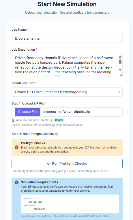
Name and describe your job
Enter a job name (lowercase letters, numbers, and hyphens) and a short description. After you upload your ZIP, the platform can suggest a name and description from your Palace
config.json.Confirm the simulation tool
Select Palace (3D Finite Element Electromagnetics) as the simulation tool.
Prepare your ZIP archive
Your ZIP must contain a Palace
config.jsonand the mesh files referenced inside it. A typical layout looks like this:your-case.zip ├── config.json └── mesh/ └── model.mshFile names can vary — the mesh paths in your JSON just have to match the files in the archive.
Step 1: Upload your ZIP
On the Start Simulation page, choose your
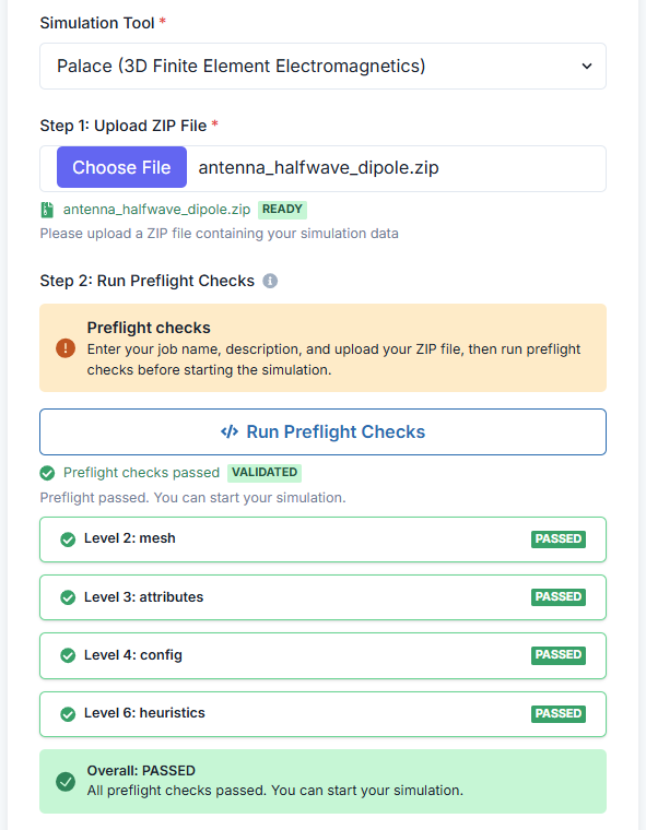
.zipfile. The upload is required before you can run preflight checks or start the job.Step 2: Run preflight checks
Click Run Preflight Checks after your job name, description, and ZIP are ready. Preflight validates your archive — including JSON syntax, Palace configuration, and mesh references — before the job is submitted. Fix any failed checks and re-run preflight until all levels pass.
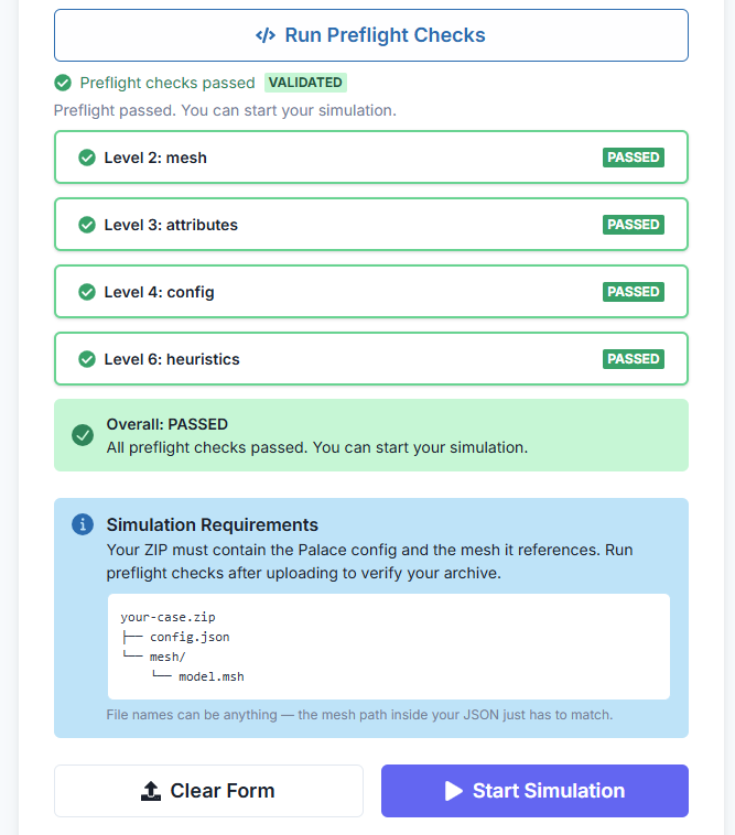
Start simulation
Once preflight passes, click Start Simulation. Your Palace job is queued and runs on cloud GPUs.
4. Monitoring Your Simulations
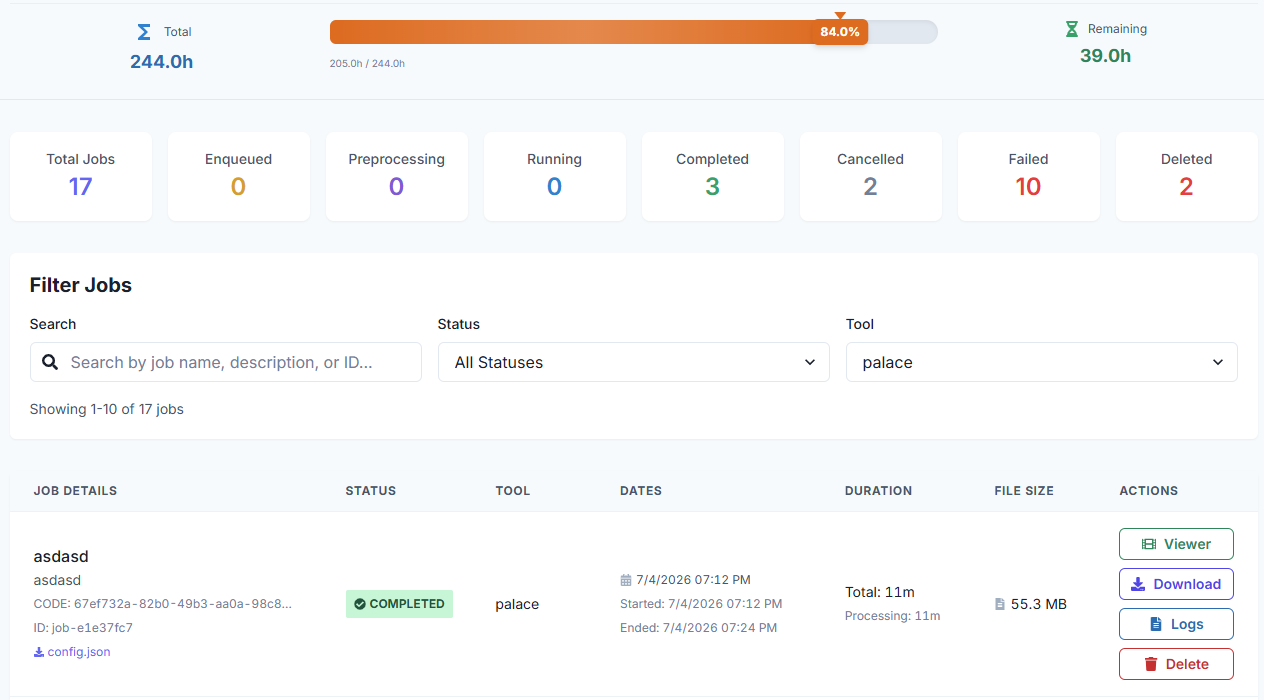
Track your simulation progress in real-time through the Jobs Portal.
Understanding Job Status
Your job is waiting in line
Performin system check, grid check, assigning resources and setting up the environment.
Simulation is actively running on GPU
Simulation finished successfully
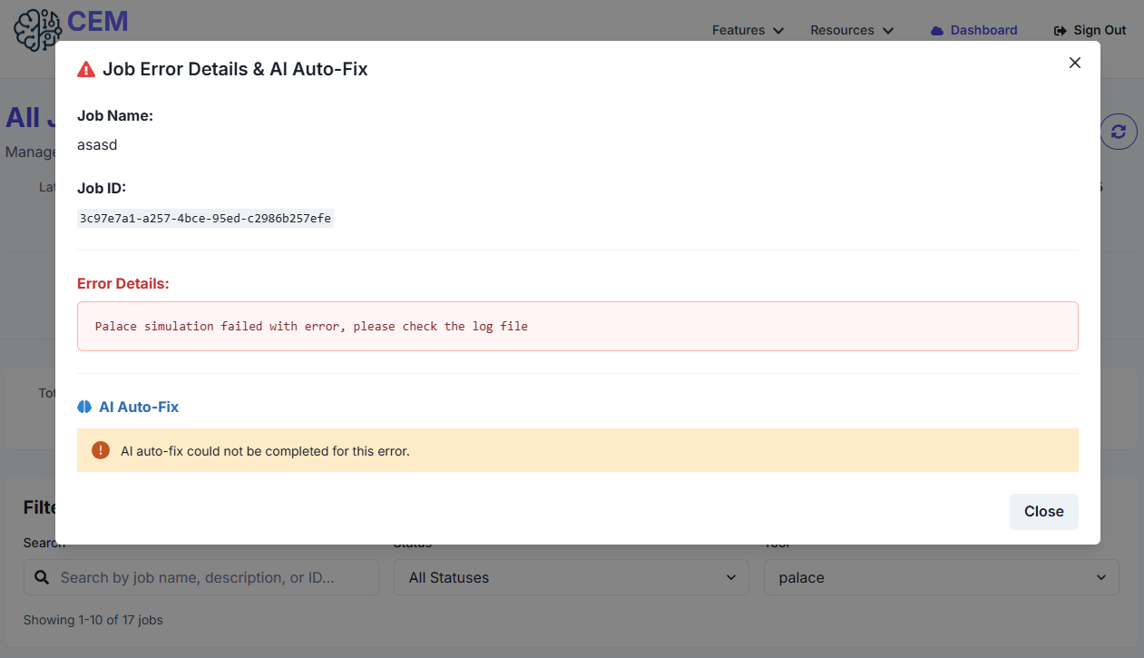
An error occurred (check logs for details)
Simulation was cancelled by the user
Key Metrics to Watch
Estimated Time Remaining (ETA)
Predicted completion time based on current progress
Duration
Total time which includes all the stages from enqueue to completion and processing time which excludes the enqueue time. Hours consumped as calculed from processing time only.
File Size
Size of the resulting files in ZIP format
Action Buttons
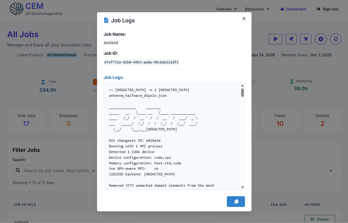
View, download, cancel, or delete the job. Logs are available for viewing.
Total Consumption
Total and reaming consumed hours are shown via the progress bar.
5. Downloading Your Results
Once your simulation completes, you can download the results for analysis.
Go to Jobs Portal
Navigate to the Jobs section from your dashboard.
Find Your Completed Job
Look for jobs with the "COMPLETED" status badge.
View Job Details
Click on the job to expand details and see output files.
Download Results
Click the "Download" button to save result files to your computer. You can also view logs directly in the browser.
What You'll Get
Simulation output files (data, visualizations)
MFC logs with detailed runtime information
Performance metrics and timing data
6. Results Visualization
Once you download the simulation results, you can use third‑party visualization tools such as VisIt (developed by Lawrence Livermore National Laboratory, LLNL) and ParaView (developed by Kitware, Inc.) to inspect and analyze your MFC output.
Visualizing MFC Results in VisIt
Viewing MFC simulation results in VisIt involves opening the MFC-generated data files (commonly .hdf5, .vtk, .xdmf, or other VisIt-friendly mesh formats), then using VisIt's plotting and analysis tools. Below is a concise guide to get you started.
What you need to do
Install a compatible VisIt version for your operating system (VisIt supports multiple platforms and data formats).
Confirm that your MFC output format is readable by VisIt. Supported options typically include VTK/VTU, XDMF, or Silo-based formats. If unsure, check the MFC build documentation.
Prepare your data path or database: point VisIt to the directory or file containing the MFC results. VisIt can also aggregate multiple time steps if the database format supports it.
Core steps in VisIt
Start VisIt and open a database
Go to File → Open File (or Open Database) and select your MFC data file or directory.
Create a plot
Choose an appropriate plot type (e.g., Pseudocolor for scalar fields, Vector for velocities).
Apply data operations
Use Expressions to compute derived quantities (e.g., velocity magnitude or custom scalars).
Time and animation
If your results contain time steps, use the Animation controls to explore temporal evolution.
Save visuals
Export images or animations via File → Save Window or Save Animation.
Visualizing MFC Results in ParaView
ParaView is another widely used post-processor for MFC outputs. The workflow is similar to VisIt but uses its own UI and readers.
Steps to open MFC results in ParaView
Install a compatible ParaView version
Download a version appropriate for your OS. Ensure that the release includes the readers you need for HPC data formats.
Determine the MFC output format
MFC commonly exports HDF5/Silo, VTK/VTU, or other database formats readable by ParaView. Check your MFC build configuration or post-processing notes if unsure.
Load the data in ParaView
Go to File → Open, then select the MFC file or directory. ParaView will load the dataset and display available fields. For multi-step outputs, ensure you open the database file (e.g., an HDF5 or VTK-based database) rather than individual time-step files.
Visualizing fields
Use the Properties panel to choose a representation (e.g., Volume, Surface, Glyphs). Adjust color maps and opacity to highlight important variables (pressure, density, velocity magnitude).
Time steps and animation
If the dataset includes multiple time steps, use ParaView's animation controls to play or scrub through time. ParaView automatically exposes time information for temporal datasets.
Derived quantities
Use the Calculator or Expressions to compute derived fields (velocity magnitude, vorticity, etc.), then visualize them alongside primary fields.
Saving and exporting results
Use File → Save Screenshot or Save Animation to export images or movies. You can also save a ParaView state file to reproduce your visualization setup.
7. Best Practices & Tips
Get the most out of NumericalAI with these expert tips:
Optimize Your Input Files
Ensure your simulation parameters are well-defined to avoid wasted compute time. Start with smaller test cases before scaling up.
Use Descriptive Names
Name your jobs clearly (e.g., "shock_tube_high_res_v3") so you can easily track multiple simulations.
Monitor Progress Regularly
Check your jobs periodically to catch any issues early. Premium users get AI-assisted error detection.
Manage Your Storage
While storage is unlimited, keep your workspace organized by deleting old jobs you no longer need.
Ready to Get Started?
Now that you know the basics, it's time to run your first simulation and experience the power of GPU-accelerated computing with AI assistance.
AI-Assisted GPU-Powered Simulations
© 2026 NumericalAI, all rights reserved. |Privacy Policy |Terms of Service |Executive brief |CEM vs HFSS |FAQ