
CEM
3D Electromagnetics
Palace Learning Guide
A beginner's guide to electromagnetic simulation — a progressive path from physical intuition to advanced Palace workflows.
Contents
How to Use This Guide
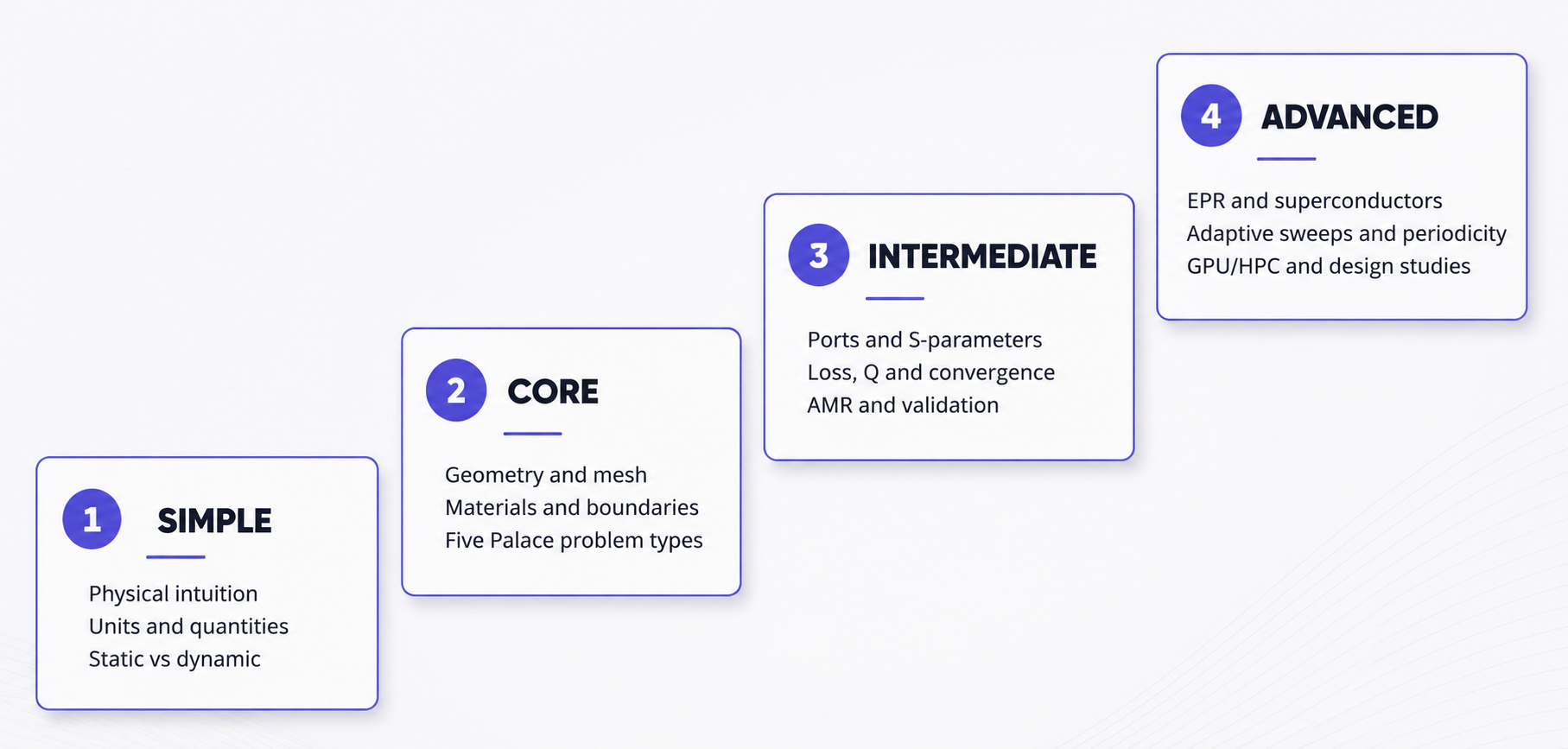
Concepts build in stages — from physical intuition to advanced Palace workflows.
This document assumes no prior background in computational electromagnetics. It first builds physical intuition, then explains the five Palace problem types, then introduces the numerical ideas needed to obtain trustworthy results. The final sections cover advanced RF, microwave, superconducting-circuit and high-performance-computing concepts.
Learning Outcomes
- Explain what Palace solves and identify when it is the right tool.
- Choose the correct Palace problem type for an engineering question.
- Understand the roles of geometry, materials, mesh attributes, boundary conditions, ports and excitations.
- Read common outputs such as capacitance matrices, inductance matrices, eigenfrequencies, quality factors and S-parameters.
- Recognize mesh, solver and modeling errors before trusting a result.
- Progress toward RF devices, antennas, resonators, transmission lines and superconducting quantum circuits.
Part I — Orientation
1. What Palace Is
Palace stands for Parallel Large-scale Computational Electromagnetics. It is an open-source, parallel finite-element solver for full-wave three-dimensional electromagnetic analysis. In practical terms, you describe an electromagnetic device using a mesh and a JSON configuration file; Palace then computes electric and magnetic fields and converts them into engineering quantities such as capacitance, inductance, resonant frequency, quality factor, voltage, current and scattering parameters.
1.1 What Palace Is Designed to Simulate
| Application field | Physical question | Typical Palace outputs |
|---|---|---|
| Electrostatics | Electric fields that do not change with time | Capacitance, charge distribution, electric-field concentration, terminal coupling |
| Magnetostatics | Magnetic fields from steady currents | Self-inductance, mutual inductance, magnetic flux and coupling |
| RF and microwave devices | Sinusoidal electromagnetic waves | Filters, couplers, resonators, waveguides, transmission lines and connectors |
| Antennas and radiation-region models | Driven electromagnetic fields in open space | Input match, near fields and radiative loss; v0.14.0 has absorbing boundaries but not the later far-zone extraction feature |
| Signal integrity | Propagation and coupling in interconnects | S-parameters, crosstalk, reflections, pulse distortion and ringing |
| Superconducting quantum hardware | Microwave modes and energy storage in superconducting circuits | Qubit/resonator modes, participation ratios, coupling and loss estimates |
| Periodic electromagnetic structures | Repeated unit cells with phase relationships | Photonic or microwave periodic structures using periodic/Floquet boundary conditions |
1.2 What Palace Does Not Directly Solve
Palace is not a general-purpose solver for every branch of physics. It does not directly solve structural stress, fluid flow, heat transfer, chemical reactions or rigid-body motion. Electromagnetic losses computed in Palace can be exported and used as inputs to thermal or structural tools, but that becomes a multiphysics workflow.
| Question | Use Palace? | Reason |
|---|---|---|
| What is the resonant frequency of a microwave cavity? | Yes | This is an electromagnetic eigenmode problem. |
| How much heat does a conductor dissipate? | Partly | Palace can estimate electromagnetic loss; a thermal solver computes temperature. |
| How does air flow around an antenna radome? | No | That is a computational-fluid-dynamics problem. |
| Will a PCB deform under vibration? | No | That is a structural-mechanics problem. |
| What are the capacitances between quantum-chip electrodes? | Yes | This is an electrostatic terminal problem. |
2. Palace v0.14.0 Problem Types
| Problem type | Question answered | Main input | Main output |
|---|---|---|---|
| Electrostatic | If I apply voltage, where is the electric field and what capacitance results? | Voltage terminals and ground | terminal-C.csv, terminal-Cinv.csv, terminal-Cm.csv |
| Magnetostatic | If steady current flows, what magnetic flux and inductance result? | Current-source surfaces | terminal-M.csv, terminal-Minv.csv, terminal-Mm.csv |
| Eigenmode | At what natural frequencies can the structure resonate, and what do the modes look like? | No external drive; search target/starting frequency | eig.csv, mode fields, Q and EPR-related files when configured |
| Driven | How does the device respond to sinusoidal excitation over frequency? | Lumped port, wave port or surface current | port-S.csv, port-V.csv, port-I.csv, fields |
| Transient | How does the device respond to a pulse or waveform over time? | Time-dependent port or current excitation | Time histories in port-V.csv and port-I.csv, fields |
A beginner’s decision tree for selecting the Palace problem type.
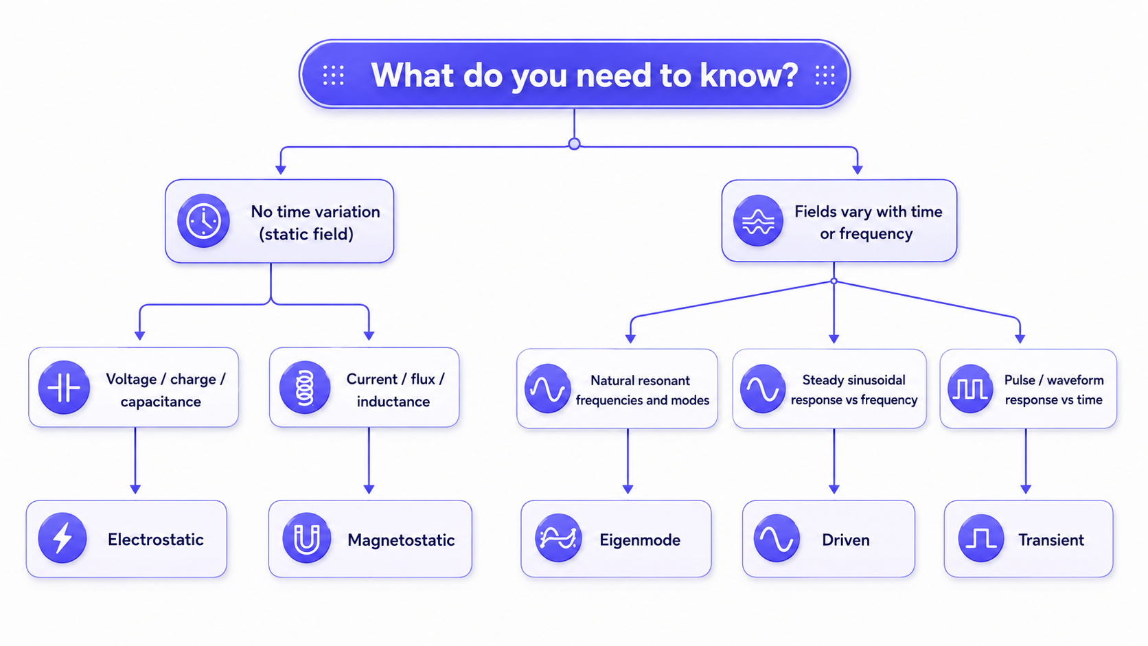
A beginner’s decision tree for selecting the Palace problem type.
3. A Complete Simulation in One Picture
Every credible simulation follows an iterative engineering workflow.
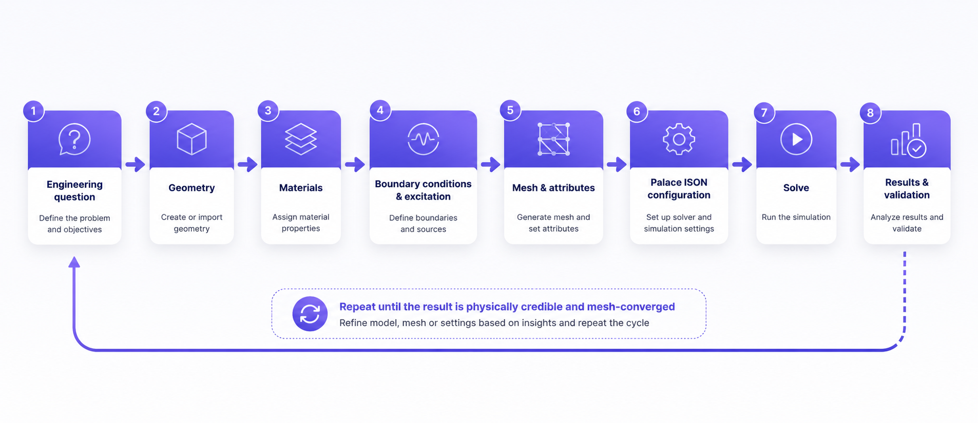
Every credible simulation is an iterative loop, from engineering question to validation.
A simulation is not merely a mesh plus a command. It begins with a precise engineering question and ends with validation. The most common beginner error is to focus on solver settings before defining the physical question, material assumptions and boundaries.
Part II — Simple Concepts
4. The Basic Electromagnetic Quantities
| Quantity | Symbol | Unit | Intuition |
|---|---|---|---|
| Electric charge | Q | coulomb (C) | The source of electric fields; positive and negative charge attract or repel. |
| Voltage | V | volt (V) | Electrical potential difference. It tells how much energy per unit charge is available. |
| Electric current | I | ampere (A) | Rate at which electric charge flows. |
| Electric field | E | volt per metre (V/m) | Force-producing field around charges and voltage differences. |
| Magnetic flux density | B | tesla (T) or Wb/m² | Magnetic field produced by currents and changing electric fields. |
| Power | P | watt (W) | Rate at which electromagnetic energy is delivered, transmitted or lost. |
| Energy | U | joule (J) | Energy stored in electric fields, magnetic fields or lumped elements. |
| Impedance | Z | ohm (Ω) | Generalized opposition to alternating current; includes resistance and reactance. |
4.1 Four Equations Worth Remembering
| Concept | Simple relation | Meaning |
|---|---|---|
| Capacitance | C = Q / V | More charge stored for the same voltage means greater capacitance. |
| Inductance | L = Φ / I | More linked magnetic flux Φ for the same current means greater inductance. |
| Impedance | Z = V / I | Voltage-to-current relationship under sinusoidal excitation. |
| Wave relation | λ = v / f | Higher frequency means shorter wavelength in the same material. |
5. Static, Frequency-Domain and Time-Domain Thinking
| Viewpoint | Assumption | Example | Palace type |
|---|---|---|---|
| Static | Nothing changes with time | A constant voltage or steady current | Electrostatic or Magnetostatic |
| Frequency domain | Assume a sinusoid that repeats forever at one frequency | RF source at 5 GHz | Driven or Eigenmode |
| Time domain | Follow the waveform step by step through time | Pulse, step, Gaussian waveform | Transient |
6. Frequency, Period, Wavelength and Phase
Frequency (f): Number of cycles per second. 1 GHz means one billion cycles per second.
Period (T): Time for one cycle. T = 1/f.
Wavelength (λ): Distance traveled during one cycle. In vacuum, λ ≈ 0.3/fGHz metres.
Phase: Position within the wave cycle. Two signals may have equal amplitude but different phase.
Propagation velocity: Speed of the wave in a material. It is slower in most dielectrics than in vacuum.
Wavelength is central to meshing. A device that is electrically small may be modeled with relatively few elements, while a structure many wavelengths long needs many more elements. Small gaps, thin layers and sharp corners can impose even stricter mesh requirements than wavelength.
7. Materials
| Material type | Key property | Effect |
|---|---|---|
| Vacuum / air | εr ≈ 1, μr ≈ 1, very low conductivity | Reference medium; waves travel fastest. |
| Perfect electric conductor (ideal metal) | Infinite conductivity idealization | No electric field inside; represented mainly through PEC boundaries. |
| Finite-conductivity metal | Large but finite conductivity | Causes conductor loss and skin effect. |
| Dielectric | Relative permittivity εr > 1 | Stores electric energy and slows waves. |
| Lossy dielectric | Permittivity plus loss tangent | Converts part of electric-field energy into heat. |
| Magnetic material | Relative permeability μr different from 1 | Changes magnetic-field storage and propagation. |
| Superconductor | Special electromagnetic response below critical conditions | Can require superconducting/London modeling and careful material assumptions. |
7.1 Permittivity, Permeability and Conductivity
Permittivity (ε): Controls how strongly a material stores electric-field energy. Relative permittivity εr is measured against vacuum.
Permeability (μ): Controls magnetic-field storage. Relative permeability μr is measured against vacuum.
Conductivity (σ): Controls how easily electric current flows and how strongly conductive loss occurs.
Loss tangent (tan δ): A convenient measure of dielectric loss under sinusoidal excitation.
8. Geometry, Domains, Surfaces and Attributes
A Palace mesh contains volume elements for material regions and surface elements for boundaries. Each region or surface is assigned an integer attribute (also called a physical tag in Gmsh workflows). The JSON file refers to these integers. The geometry name may help humans, but Palace ultimately uses the numerical attributes.
9. Boundary Conditions
| Boundary | Meaning | Typical use |
|---|---|---|
| PEC | Perfect electric conductor | Ideal metal surface; tangential electric field is zero. |
| PMC | Perfect magnetic conductor / magnetic insulation | A symmetry-like boundary; tangential magnetic field is zero. |
| Ground | Zero electric potential | Reference voltage for electrostatic simulations. |
| ZeroCharge | No normal electric flux | Natural insulation boundary for electrostatics. |
| Impedance | Relationship between tangential electric and magnetic fields | Represents an R/L/C-like surface behavior. |
| Absorbing | Approximate open-region boundary | Reduces artificial reflections at the truncated outer boundary. |
| Conductivity | Finite-conductivity surface | Models conductor loss without meshing deep into a thick conductor. |
| Periodic | Fields match across repeated boundaries | Represents a repeated unit cell. |
| Floquet periodic | Periodic match with a phase shift | Represents oblique or phase-progressive periodic behavior. |
10. Terminals, Lumped Ports, Wave Ports and Current Sources
| Object | Intuition | Typical use |
|---|---|---|
| Terminal | A conductor held at a voltage for electrostatic matrix extraction | Capacitance between conductors |
| Surface current source | A prescribed current-carrying surface | Magnetostatic inductance or driven excitation |
| Lumped port | A compact circuit-like connection with a direction and impedance | PCB gap, CPW feed, qubit junction representation |
| Wave port | A boundary excited using a computed cross-sectional mode | Coaxial cable, rectangular waveguide, complex transmission line |
Part III — Core Palace Concepts
11. Finite Element Method — An Intuitive View
The finite element method (FEM) breaks a complicated electromagnetic domain into many small elements. Palace represents the unknown field inside each element using polynomial basis functions and then assembles the local contributions into a large system of equations. Solving that system gives an approximation to the field throughout the model.
| FEM idea | Plain-language meaning |
|---|---|
| Discretization | Replace an infinite number of possible field values with a finite set of unknowns. |
| Element | A small tetrahedron, hexahedron, prism or other mesh cell. |
| Basis function | A mathematical shape used to represent how the field varies inside an element. |
| Order p | Polynomial complexity inside each element; higher order can represent smoother variation more accurately. |
| Degrees of freedom | The numerical unknowns solved by Palace. |
| Assembly | Combine element-level equations into the global system. |
| Linear solve / eigensolve | Numerically solve for fields or resonant modes. |
12. Mesh Fundamentals
The mesh is one of the strongest determinants of simulation accuracy, runtime and memory. A coarse mesh may run quickly but miss important field variation. An excessively fine mesh may consume all available memory without improving the result meaningfully.
| Mesh concept | Meaning | Practical advice |
|---|---|---|
| Global size | Overall element size throughout the model | Start coarse for debugging, then refine. |
| Local refinement | Smaller elements near gaps, edges, junctions or ports | Often more efficient than refining everything. |
| Element quality | Shape regularity of elements | Very distorted elements can hurt accuracy and solver convergence. |
| Wavelength resolution | Elements per wavelength | Dynamic problems need enough spatial resolution; higher-order elements change the rule. |
| Geometric resolution | Elements across thin or narrow features | A feature must be represented by enough elements to affect the solution correctly. |
| Curved/high-order mesh | Curved element geometry | Useful for cavities, coaxial structures and smooth conductors. |
12.1 Mesh Attributes
Domain attributes identify material volumes; boundary attributes identify surfaces. In Palace 0.14.0, attribute integers should be positive and do not have to be contiguous. The JSON keyword "Attributes" selects the tagged regions to which a material, boundary condition, port or postprocessing request applies.
Example concept only:
"Domains": {
  "Materials": [
    {"Attributes": [1], "Permeability": 1.0, "Permittivity": 11.45},
    {"Attributes": [2], "Permeability": 1.0, "Permittivity": 1.0}
  ]
},
"Boundaries": {
  "PEC": {"Attributes": [10, 11]},
  "Absorbing": {"Attributes": [20], "Order": 1}
}
13. Units and the Model Length Scale L0
Palace nondimensionalizes the problem internally. The configuration parameter Model.L0 tells Palace what one mesh coordinate unit means in metres. For example, if the mesh coordinates are in micrometres, L0 = 1e-6. If coordinates are in millimetres, L0 = 1e-3. Incorrect L0 can shift resonant frequencies and all dimensional outputs by orders of magnitude.
| Mesh coordinate unit | Model.L0 |
|---|---|
| Mesh drawn in metres | 1.0 |
| Mesh drawn in millimetres | 1.0e-3 |
| Mesh drawn in micrometres | 1.0e-6 |
| Mesh drawn in nanometres | 1.0e-9 |
14. Palace JSON Configuration
A Palace configuration is a structured JSON file. The exact sections vary by problem type, but the following mental map is useful.
| Top-level section | Purpose |
|---|---|
| Problem | Problem type, output directory and verbosity |
| Model | Mesh file, length scale and refinement options |
| Domains | Material properties and domain postprocessing |
| Boundaries | PEC/PMC, terminals, ports, current sources, absorbing and other surface conditions |
| Solver | Finite-element order, problem-specific settings, linear/eigen solver settings, device/backend and output controls |
{
  "Problem": {
    "Type": "Eigenmode",
    "Output": "postpro"
  },
  "Model": {
    "Mesh": "model.msh",
    "L0": 1.0e-3
  },
  "Domains": {
    "Materials": [...]
  },
  "Boundaries": {
    "PEC": {...}
  },
  "Solver": {
    "Order": 1,
    "Eigenmode": {...}
  }
}
15. Running Palace 0.14.0
The standard wrapper command is:
palace -np <NUM_PROCS> config.json
To keep the console output and save it for later diagnosis:
palace -np 4 config.json 2>&1 | tee palace.log
The -np value controls MPI processes. In a GPU run, the correct number of MPI processes depends on the number of GPUs, the build, memory limits and the model. More processes are not automatically faster.
16. Core Problem Type 1 — Electrostatic
Electrostatic simulation assumes the electric field is constant in time. Palace applies a unit voltage to each terminal in turn while the others and the ground are held at zero, then constructs capacitance matrices.
| Aspect | Explanation |
|---|---|
| Use it for | Capacitance extraction, field concentration, conductor coupling, electrodes, sensors and quantum-chip capacitance |
| Main objects | Dielectric domains, terminal boundaries, ground and optional zero-charge boundaries |
| Primary output | Maxwell capacitance matrix terminal-C.csv; inverse and mutual forms are also written |
| Visual output | Electric potential V, electric field E, electric energy density |
| First example | Two conducting spheres or a parallel-plate capacitor |
16.1 How to Read a Capacitance Matrix
Diagonal entries primarily represent self-capacitance relative to the reference, while off-diagonal entries represent coupling between terminals. Sign conventions depend on the matrix form. Always verify units and the precise matrix definition before comparing against another tool.
16.2 Common Electrostatic Mistakes
- No ground or reference boundary, leaving the potential undefined.
- A conductor surface split into multiple attributes but only one attribute is assigned as the terminal.
- Incorrect dielectric permittivity.
- Mesh too coarse in narrow gaps where the electric field is concentrated.
- Confusing Maxwell capacitance, mutual capacitance and two-terminal capacitance.
17. Core Problem Type 2 — Magnetostatic
Magnetostatic simulation assumes steady current. Palace excites current-source surfaces and computes magnetic fields and inductance matrices.
| Aspect | Explanation |
|---|---|
| Use it for | Coils, current loops, mutual coupling, inductors, packages and interconnect inductance |
| Main objects | Current-source boundaries, conducting paths, material permeability and magnetic-insulation/PEC-like conditions |
| Primary output | Inductance matrix terminal-M.csv; inverse and mutual forms are also written |
| Visual output | Magnetic flux density B, vector potential A, magnetic energy density |
| First example | Concentric rings carrying current |
17.1 Common Magnetostatic Mistakes
- An open or incomplete current path.
- Incorrect source direction or surface orientation.
- Using unsuitable boundary conditions around the current-carrying region.
- Ignoring magnetic material permeability.
- Mesh too coarse near conductors or in small magnetic gaps.
18. Core Problem Type 3 — Eigenmode
An eigenmode simulation finds the structure’s natural electromagnetic resonances. No external drive is required. Each mode has an eigenfrequency, a field pattern and, when loss is included, a quality factor.
| Aspect | Explanation |
|---|---|
| Use it for | Cavities, resonators, filters, package modes, readout resonators and superconducting quantum circuits |
| Main objects | Closed or lossy boundaries, materials, optional lumped elements and a target/search frequency |
| Primary output | eig.csv containing eigenfrequencies, Q values and numerical error measures |
| Visual output | Electric and magnetic mode shapes and energy density |
| First example | Eigenmodes of a conducting cylinder or cavity |
A resonant response has a centre frequency and a bandwidth; their ratio gives an intuitive Q.
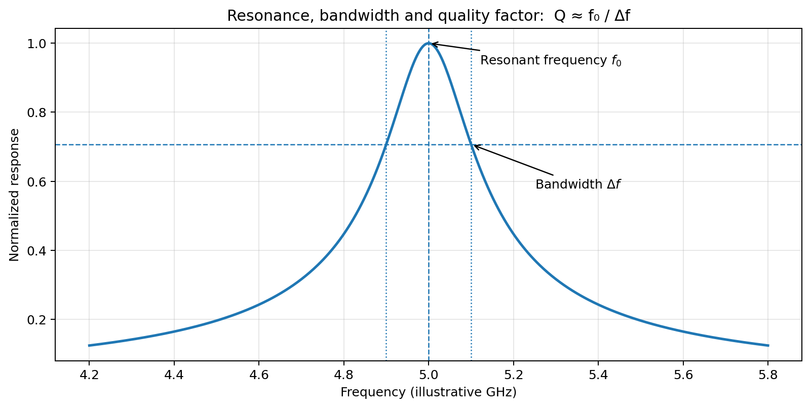
Resonance, bandwidth and quality factor: Q ≈ f₀ / Δf.
18.1 Mode Identification
A mode number is not a permanent physical label. Mesh changes, target frequency and solver settings can reorder computed modes. Identify modes using field patterns, symmetry, energy distribution and continuity across parameter sweeps—not only by row number.
18.2 Common Eigenmode Mistakes
- Searching around the wrong frequency because geometry units or L0 are wrong.
- Requesting too few modes and missing the mode of interest.
- Mistaking a spurious, port-localized or box mode for the intended device mode.
- Comparing mode 1 in two designs without checking field-pattern similarity.
- Reporting Q without stating which loss mechanisms were included.
19. Core Problem Type 4 — Driven Frequency Domain
A driven simulation applies a sinusoidal source at selected frequencies and solves the steady-state response. This is the main Palace workflow for S-parameters, filters, transmission lines, crosstalk and input matching.
| Aspect | Explanation |
|---|---|
| Use it for | S11/S21, impedance matching, filters, couplers, waveguides, antennas and frequency response |
| Main objects | Lumped port, wave port or surface-current excitation; frequency samples or sweep |
| Primary output | port-S.csv plus port-V.csv, port-I.csv and optional fields |
| Visual output | Complex E and B fields, Poynting vector, energy density and surface currents |
| First example | Signal propagation through a coaxial cable |
19.1 A Frequency Sweep
A frequency sweep solves the same physical model at multiple frequencies. A coarse sweep is useful for finding broad behavior. A fine sweep is needed near narrow resonances. Palace 0.14.0 supports uniform and flexible sample definitions, plus an adaptive fast frequency sweep using a reduced-order model.
19.2 Common Driven-Simulation Mistakes
- Exciting the wrong port or more ports than intended.
- Incorrect reference impedance or port geometry.
- Frequency range does not include the resonance or cutoff region.
- Absorbing boundary placed too close to a radiating structure.
- Interpreting S21 without checking whether both ports support the intended mode.
20. Core Problem Type 5 — Transient
A transient simulation starts from rest and follows the electromagnetic response to a time-dependent excitation. It is useful for pulses, propagation delay, ringing and broadband effects viewed in time.
| Aspect | Explanation |
|---|---|
| Use it for | Pulse propagation, reflections, ringing, crosstalk in time and impulse-like studies |
| Main objects | Time-dependent lumped-port or surface-current excitation, total time and integration settings |
| Primary output | Time histories in port-V.csv and port-I.csv |
| Visual output | Field snapshots over time |
| First example | A pulse traveling through a coaxial cable or transmission line |
20.1 Time Step and Duration
The time step must be small enough to resolve the highest important frequency and numerical dynamics. The total duration must be long enough for the pulse to reach the observation point and for ringing to decay. Palace 0.14.0 also supports adaptive time stepping through CVODE and ARKODE integrators.
20.2 Common Transient Mistakes
- Simulation time ends before the signal reaches the output.
- The excitation pulse has bandwidth far beyond what the mesh can resolve.
- Output is saved too infrequently, hiding the waveform shape.
- A reflected pulse is mistaken for numerical noise.
- Using dielectric loss tangent assumptions where the transient formulation requires conductivity-based loss treatment.
Part IV — Intermediate Concepts
21. Impedance and Matching
Impedance describes how voltage and current relate under alternating excitation. A source transfers power efficiently when the device and transmission system are appropriately matched. A discontinuity in impedance produces reflections.
Resistance: Dissipates energy as heat.
Reactance: Stores and returns energy through electric or magnetic fields.
Characteristic impedance: The voltage-to-current relation of a propagating transmission-line mode.
Reference impedance: The impedance against which S-parameters are normalized, often 50 Ω in RF systems.
22. S-Parameters
| Parameter | Meaning | Interpretation |
|---|---|---|
| S11 | Reflection at port 1 | How much of the input returns to the source. More negative dB usually means a better match. |
| S21 | Transmission from port 1 to port 2 | How much signal reaches port 2. |
| S12 | Transmission from port 2 to port 1 | Reverse transmission or isolation behavior. |
| S22 | Reflection at port 2 | Output-port match. |
S-parameters are complex numbers. Magnitude shows how much; phase shows timing or phase shift. In dB, magnitude is commonly reported as 20 log10|Sij|. A value of −20 dB corresponds to a magnitude of 0.1, not a power fraction of 20%.
23. Resonance and Quality Factor Q
A resonator stores energy and exchanges it between electric and magnetic forms. The quality factor Q measures how slowly stored energy decays relative to the oscillation rate. High Q means a narrow resonance and low loss; low Q means a broad resonance and faster decay.
| Q type | Meaning |
|---|---|
| Loaded Q | Includes internal loss and external coupling to ports. |
| Internal Q | Loss inside materials, conductors and interfaces. |
| External/coupling Q | Energy leakage through ports or radiation channels. |
| Dielectric Q contribution | Related to electric energy in lossy dielectric regions. |
| Conductor Q contribution | Related to surface-current loss in finite-conductivity conductors. |
24. Loss Mechanisms
| Loss mechanism | Modeling route | Where it matters |
|---|---|---|
| Dielectric loss | Loss tangent or conductivity in dielectric volumes | Regions with strong electric energy |
| Conductor loss | Finite conductivity or surface impedance | Regions with strong surface current |
| Radiative loss | Energy escaping through open boundaries | Antennas, cavities with apertures, package leakage |
| Port coupling loss | Energy leaving through ports | Readout lines, feedlines and external coupling |
| Interface loss | Thin lossy layers at material interfaces | Important in superconducting quantum circuits |
A Q value is meaningful only when the included losses are stated. An ideal PEC cavity with lossless dielectric may have an effectively infinite physical Q, while the numerical eigensolver still reports finite error estimates that must not be confused with physical loss.
25. Field Visualization and Postprocessing
Palace can write field data for ParaView. Common quantities include electric field E, magnetic flux density B, potential V, magnetic vector potential A, electric and magnetic energy density, Poynting vector, surface charge and surface current. Palace 0.14.0 also writes problem-specific CSV measurements such as eigenfrequencies, port voltage/current and matrix data.
| Visualization | Question answered | Caution |
|---|---|---|
| Field magnitude | Where is the field strongest? | Useful for hotspots but hides direction and phase. |
| Real/imaginary components | What is the complex field phase? | Relevant in frequency-domain results. |
| Vector glyphs | Which direction does the field point? | Use sparingly; dense glyphs can be misleading. |
| Energy density | Where is electromagnetic energy stored? | Useful for resonators, EPR and loss analysis. |
| Surface current | Where does current concentrate on conductors? | Useful for conductor loss and feed understanding. |
| Poynting vector | Where does electromagnetic power flow? | Useful for propagation and radiation. |
26. Mesh Convergence
A result is mesh-converged when further sensible mesh refinement changes the quantity of interest by less than an agreed tolerance. Convergence should be tested on the engineering quantity you plan to report—not merely on the solver residual.
| Problem type | Convergence quantity |
|---|---|
| Electrostatic | Selected capacitance entries and peak/average field in important regions |
| Magnetostatic | Selected self and mutual inductances |
| Eigenmode | Frequency, Q and energy participation of the target mode |
| Driven | S11/S21 at key frequencies, resonance location and bandwidth |
| Transient | Arrival time, peak voltage and ringing envelope |
26.1 A Basic Convergence Procedure
- Run a coarse model that is small enough to debug quickly.
- Refine the mesh globally or locally in physically important regions.
- Repeat the simulation without changing the physical model.
- Compare the key quantity of interest.
- Continue until the change is below your tolerance and the field pattern remains physically consistent.
- Record element count, degrees of freedom, order, runtime and memory for every level.
27. Polynomial Order: h-Refinement and p-Refinement
Reducing element size is called h-refinement. Increasing the finite-element polynomial order is p-refinement. Both can increase accuracy, but their cost and effectiveness differ. Smooth fields in well-shaped elements often benefit from higher order; singular corners, thin gaps and abrupt material changes often still require local h-refinement.
28. Adaptive Mesh Refinement (AMR)
AMR uses an error indicator from the computed solution to refine selected elements. Palace 0.14.0 supports solution-based AMR for all problem types except Transient. AMR is powerful, but it does not replace physical judgment: the error estimator may refine a mathematically difficult region that is irrelevant to your design objective, or it may need help through initial local refinement.
29. Solver Convergence vs Physical Accuracy
| Statement | True or false? | Explanation |
|---|---|---|
| The linear residual is small, so the simulation is accurate. | False | The algebraic system may be solved accurately for a physically wrong or under-resolved model. |
| The fields look smooth, so the mesh is adequate. | False | Plot interpolation can hide under-resolution. |
| A result that agrees with an analytic limit is more credible. | True | Analytic, measured or benchmark comparison provides independent validation. |
| More MPI ranks always improve speed. | False | Communication and coarse-solver cost can dominate. |
| A finer mesh always fixes a wrong boundary condition. | False | It converges to the wrong physical problem more accurately. |
30. Verification and Validation
Verification: Did we solve the mathematical model correctly? Examples: mesh convergence, solver tolerance and code benchmark.
Validation: Does the mathematical model represent the real device? Examples: comparison with measurement or a trusted experiment.
For an engineering report, include both. A highly converged result can still be invalid if the material permittivity, conductor thickness, connector geometry or environmental boundary is wrong.
Part V — Advanced Concepts
31. Lumped Ports vs Numeric Wave Ports
| Port type | How it works | Best use |
|---|---|---|
| Lumped port | Assumes a simple localized field direction and equivalent circuit impedance | Compact feeds, gaps, CPW connections and lumped RLC elements |
| Numeric wave port | Solves a two-dimensional modal problem on the port cross-section | Coaxial lines, waveguides and arbitrary transmission-line cross-sections |
A wave port is usually more physically descriptive for a true propagating cross-section, but it has stricter geometric and meshing requirements. The port must lie on an outer boundary and the cross-section must be large and clean enough to support the intended mode.
32. Adaptive Fast Frequency Sweeps
A conventional driven sweep solves the large full-order system at every requested frequency. An adaptive sweep solves selected frequencies, constructs a reduced-order model and uses it to approximate the response over the band. Palace activates this behavior through a nonzero AdaptiveTol.
| When it helps | When to be cautious |
|---|---|
| Many frequency samples over a band | Very sharp or complex resonances that are difficult for the reduced model |
| Repeated design studies with similar response structure | Insufficient validation points |
| Large models where each full solve is expensive | Frequency-dependent effects not represented correctly in the selected model |
33. Multiple Excitations
Palace 0.14.0 can represent multiple excitation indices in one driven configuration and simulate them consecutively. This is useful for generating multiple columns of a multiport response, but output-column naming and S-parameter behavior must be interpreted carefully. Automated workflows should explicitly map excitation index, source port and output columns.
34. Periodic and Floquet-Periodic Boundaries
Periodic boundaries model a repeated unit cell by matching fields on a donor and receiver surface. Floquet-periodic boundaries introduce a phase shift between repeated cells. Palace 0.14.0 added exact periodic and Floquet phase-delay constraints. This feature is a boundary condition within supported problem types; it is not the later standalone FloquetPort feature.
- Donor and receiver surface meshes must match exactly for configuration-specified periodic matching in v0.14.0.
- The translation or rotation relationship must be correct.
- The Floquet wave vector controls the phase progression between cells.
- A sign or coordinate-system mistake can reverse the intended propagation phase.
35. Energy Participation Ratio (EPR)
EPR describes how much of a mode’s energy is stored in a particular element or material region. In superconducting-circuit analysis, Palace can use lumped inductive ports representing linearized Josephson junctions and compute inductive participation data for circuit quantization.
| EPR concept | Meaning |
|---|---|
| Mode energy | Total electromagnetic energy of the eigenmode |
| Element participation | Fraction associated with a selected lumped inductive element |
| Bulk participation | Fraction of electric energy in a dielectric volume |
| Interface participation | Fraction associated with a thin lossy interface model |
| Use in Q estimation | Participation multiplied by loss assumptions gives a contribution to inverse Q |
36. Superconducting Electromagnetics
Superconductors are not always equivalent to ideal PEC surfaces. Depending on frequency, temperature, film thickness and the desired accuracy, one may need finite penetration depth, kinetic inductance or a London-equation model. Palace includes superconducting modeling capabilities, but the correct parameters must come from the physical fabrication stack and operating conditions.
| Approximation | When it may be reasonable | What it misses |
|---|---|---|
| PEC | Early geometry debugging or thick, low-loss conductors when kinetic effects are negligible | Penetration, kinetic inductance and conductor loss |
| Surface impedance | Thin-film or frequency-domain loss approximation | Detailed field variation through thickness |
| London/superconducting domain model | When penetration depth and kinetic inductance matter | Still requires accurate material parameters and geometry |
37. Surface Impedance, Skin Depth and Thin Conductors
At high frequency, current concentrates near a conductor surface. The skin depth becomes small, making full volumetric meshing of a thick conductor wasteful. A finite-conductivity or impedance boundary can approximate the surface behavior when its assumptions are valid. Very thin films, superconductors and multilayers may require more specialized treatment.
38. Symmetry
Symmetry can reduce a model to a fraction of the full geometry, saving memory and runtime. PEC and PMC-like symmetry planes select different field parities. A symmetry plane is valid only if geometry, materials, boundaries, excitation and the desired mode all share that symmetry.
39. High-Order Elements and Curved Geometry
High-order finite elements can represent smooth fields accurately with fewer elements than first-order methods, especially in wave problems. Curved high-order geometry also reduces staircase error on cylindrical and smoothly curved surfaces. The trade-off is more degrees of freedom per element and greater implementation complexity.
40. GPU, MPI and HPC Concepts
| Term | Meaning |
|---|---|
| MPI rank | An independent parallel process owning part of the mesh |
| Thread | A shared-memory execution unit inside a process |
| GPU device | Accelerator executing suitable finite-element and linear-algebra operations |
| Domain decomposition | Splitting the mesh among MPI ranks |
| Partial assembly | Apply finite-element operators without building the full global matrix |
| Preconditioner | Transforms the linear system so an iterative solver converges faster |
| Coarse solve | Global low-resolution component that can limit scalability and memory |
Palace 0.14.0 supports NVIDIA and AMD GPU acceleration and multi-GPU parallelism when built with the required dependencies. Performance depends on problem type, finite-element order, partial assembly, solver/preconditioner, mesh partitioning and the ratio of computation to communication.
40.1 Memory Planning
- Record total elements, degrees of freedom and polynomial order.
- Leave memory headroom for mesh refinement, coarse matrices, eigensolver subspaces and output fields.
- Do a small run before launching a production model.
- Avoid saving every field at every frequency or time step unless necessary.
- Treat GPU memory and host memory as separate constraints.
41. Design Sweeps, Sensitivity and Uncertainty
A single simulation answers one model. Engineering design requires understanding how results change with geometry and material uncertainty. Examples include substrate permittivity tolerance, conductor width, gap size, junction inductance and package dimensions.
| Method | Purpose |
|---|---|
| Parameter sweep | Vary one or more inputs and repeat the simulation. |
| Sensitivity | Estimate how strongly an output changes with an input. |
| Tolerance analysis | Study manufacturing variation around the nominal design. |
| Optimization | Search parameters to meet targets such as resonance, bandwidth or coupling. |
| Surrogate model | Train a faster approximation from a carefully designed simulation dataset. |
42. Multiphysics Coupling
Palace results can feed other solvers. For example, conductor and dielectric loss can become heat sources in a thermal solver; thermal expansion can then update geometry; stress and temperature can change material properties. Such workflows require explicit data transfer, unit consistency and validation at every interface.
43. Version-Specific Feature Awareness
| Category | Examples |
|---|---|
| Available in 0.14.0 | Five problem types, adaptive transient stepping, flexible frequency samples, multiple driven excitations, exact/Floquet periodic boundaries, GPU support, AMR except transient |
| Added after 0.14.0 | Standalone BoundaryMode solver and general 2D support (0.17), Floquet ports (0.17), far-zone field extraction (0.15), newer runtime schema validation (0.16), resolved configuration output through --dry-run (0.17) |
Part VI — Practical Learning Roadmap
44. Recommended 12-Week Sequence
| Week | Theme | Concepts | Deliverable |
|---|---|---|---|
| 1 | Simulation mindset | Engineering question, assumptions, geometry/material/boundary/output workflow | Explain a model without using software. |
| 2 | EM fundamentals | Voltage, current, E, B, energy, frequency, wavelength and phase | Solve simple unit and wavelength exercises. |
| 3 | Mesh and Palace structure | Gmsh attributes, domains, boundaries, L0 and JSON sections | Inspect an example mesh and map all tags. |
| 4 | Electrostatics | Terminals, ground, capacitance matrix and field concentration | Run two spheres or parallel plates. |
| 5 | Magnetostatics | Current sources, flux and inductance matrix | Run concentric rings. |
| 6 | Eigenmodes | Resonance, field patterns, Q and target frequency | Run a cylindrical cavity. |
| 7 | Driven RF | Lumped/wave ports, sweeps and S-parameters | Run a coaxial transmission example. |
| 8 | Transient | Pulse waveform, time step, duration, delay and reflection | Run a coaxial pulse. |
| 9 | Loss and Q | Dielectric, conductor, radiation and coupling loss | Compare ideal and lossy models. |
| 10 | Accuracy | Mesh convergence, order, AMR, solver tolerance and validation | Produce a convergence table. |
| 11 | Performance | MPI, GPU, partial assembly, output cost and memory | Benchmark 1, 2 and 4 ranks or available GPU settings. |
| 12 | Capstone | Select RF/quantum application and write a reproducible report | Complete one validated multi-stage workflow. |
45. Ordered Hands-On Exercises
Exercise 1 — Capacitance of Two Conductors
Problem type: Electrostatic
Objective: Learn terminals, ground, dielectric permittivity, electric field and capacitance.
- Run the official spheres example or construct two parallel plates.
- Visualize potential and electric-field magnitude.
- Change separation and predict whether capacitance rises or falls.
- Refine the mesh in the gap and make a convergence table.
Deliverable: A one-page report with geometry, assumptions, C value, field plot and convergence result.
Exercise 2 — Inductance of Current Loops
Problem type: Magnetostatic
Objective: Learn current sources, magnetic flux, self-inductance and mutual inductance.
- Run the official rings example.
- Reverse one current direction and observe the sign/coupling change.
- Change ring spacing and predict mutual inductance.
- Check mesh convergence around conductors.
Deliverable: Inductance matrix plus a magnetic-field visualization and interpretation.
Exercise 3 — Resonant Modes of a Cavity
Problem type: Eigenmode
Objective: Learn target frequency, mode shape, frequency convergence and Q interpretation.
- Run the official cylinder example.
- Request multiple modes and classify them by field pattern.
- Change a cavity dimension and predict frequency change.
- Compare first-order and higher-order or refined-mesh results.
Deliverable: A mode table containing frequency, mode description, mesh size and numerical error.
Exercise 4 — Coaxial Transmission
Problem type: Driven and Transient
Objective: Learn wave/lumped ports, S11/S21, propagation delay and reflections.
- Run the official coaxial example in driven mode.
- Plot S11 and S21 over frequency.
- Introduce an impedance discontinuity and observe reflection.
- Run a pulse and measure arrival/reflection time.
Deliverable: Frequency and time-domain plots with a physical explanation.
Exercise 5 — Coplanar Waveguide / Quantum-Device Preparation
Problem type: Driven and Eigenmode
Objective: Learn field concentration, ports, substrate effects, resonators and participation concepts.
- Run the official CPW example.
- Change substrate permittivity and observe propagation/resonance changes.
- Refine gaps and conductor edges.
- Add a simple lumped inductive element only after the baseline model is validated.
Deliverable: A reproducible CPW report and a list of assumptions needed before an EPR model.
46. Suggested Capstone Projects
| Project | Palace workflow | Main outputs | Difficulty |
|---|---|---|---|
| RF filter/resonator | Eigenmode + Driven | Resonant frequencies, S11/S21, bandwidth and Q | Moderate |
| Coaxial connector discontinuity | Driven + Transient | Reflection, insertion loss and pulse echo | Moderate |
| Package or enclosure mode study | Eigenmode | Unwanted cavity modes and field hotspots | Moderate |
| CPW crosstalk | Driven | Near-end/far-end coupling and S-parameter matrix | Moderate–high |
| Simplified transmon-readout structure | Eigenmode + EPR | Mode frequencies, junction participation and coupling | High |
| Periodic unit cell | Eigenmode/Driven with Floquet periodic boundaries | Dispersion or phase-progressive response | High |
47. What a Good Simulation Report Contains
- Engineering question and acceptance criteria
- Palace version, build/backend and command used
- Geometry source and dimensional units
- Mesh file format, element count, attributes and refinement strategy
- Material properties with sources and operating conditions
- Boundary conditions, ports, directions and excitations
- Solver order, frequency/time settings and convergence tolerances
- Hardware, MPI ranks, GPU device, runtime and memory
- Results with units and field/S-parameter plots
- Mesh-convergence and validation evidence
- Known limitations and recommended next step
Part VII — Checklists and Glossary
48. Pre-Run Checklist
| Area | Check |
|---|---|
| Question | Is the required output explicitly defined? |
| Problem type | Is Electrostatic/Magnetostatic/Eigenmode/Driven/Transient the correct formulation? |
| Version | Does the input syntax match Palace 0.14.0? |
| Geometry | Are all important gaps, thicknesses, conductors and openings represented? |
| Units | Is Model.L0 correct? |
| Mesh | Are element quality, local refinement and attribute tags verified? |
| Materials | Are εr, μr, conductivity and loss values appropriate for frequency and temperature? |
| Boundaries | Does every outer and internal surface have the intended physical meaning? |
| Ports/sources | Are index, attributes, direction, impedance and excitation correct? |
| Solver | Are order, frequency/time range, target and output saving reasonable? |
| Resources | Does the model fit host and GPU memory with headroom? |
| Output directory | Is it writable and unique for this run? |
49. Post-Run Credibility Checklist
| Area | Check |
|---|---|
| Completion | Did Palace exit normally without warnings that affect physics? |
| Fields | Do field patterns match physical intuition and symmetries? |
| Units | Are frequencies, dimensions, voltages, currents and energies plausible? |
| Conservation | Are reflected, transmitted and lost powers physically consistent where applicable? |
| Modes | Is the target mode identified by field pattern, not only index? |
| Convergence | Is the reported quantity stable under mesh/order refinement? |
| Validation | Does it agree with an analytic estimate, benchmark, measurement or trusted solver? |
| Sensitivity | Are conclusions robust to uncertain material and geometry parameters? |
| Documentation | Can another person reproduce the run from the saved files? |
50. Beginner Troubleshooting Map
| Symptom | Likely causes | First action |
|---|---|---|
| Palace cannot read the mesh | File format/version, damaged file, unsupported elements, wrong path | Open the mesh in Gmsh/ParaView; inspect $MeshFormat; test a minimal mesh. |
| Boundary attribute not found | JSON tag does not exist or surface was not exported | List mesh physical attributes and compare exactly. |
| Frequency is orders of magnitude wrong | Incorrect L0 or geometry scale | Measure a known dimension and verify units. |
| No expected resonance | Wrong target/range, mode excluded by symmetry, port/boundary error | Broaden search; remove symmetry; inspect fields. |
| S11/S21 looks unphysical | Port direction, impedance, mode or normalization problem | Validate a uniform transmission-line baseline first. |
| Linear solver stalls | Poor mesh, difficult material contrast, unsuitable preconditioner or insufficient memory | Simplify model, reduce order, inspect quality and solver settings. |
| CUDA out of memory | Too many degrees of freedom, eigensolver subspace or saved fields | Coarsen/refine selectively, reduce modes/order/output, change decomposition. |
| Result changes greatly with refinement | Model is not converged or has singular/high-field features | Refine locally and report convergence rather than a single value. |
51. Essential Glossary
| Term | Definition |
|---|---|
| Absorbing boundary | Approximate open-space condition intended to reduce reflections from the truncated model boundary. |
| Adaptive mesh refinement (AMR) | Automatic local refinement based on an estimated numerical error. |
| Attribute | Integer tag assigned to a mesh domain or boundary and referenced in the JSON file. |
| Bandwidth | Frequency range over which a device meets a chosen response criterion. |
| Boundary condition | Mathematical rule specifying how fields behave on a surface. |
| Capacitance matrix | Relation between terminal charges and terminal voltages. |
| Characteristic impedance | Voltage-to-current ratio of a propagating transmission-line mode. |
| Conductivity | Measure of how easily current flows through a material. |
| Convergence | Stability of the quantity of interest as numerical resolution is improved. |
| Cutoff frequency | Lowest frequency at which a waveguide mode can propagate. |
| Degree of freedom | Unknown numerical coefficient solved by the finite-element method. |
| Dielectric | Material that stores electric energy and polarizes in an electric field. |
| Driven simulation | Steady-state response to sinusoidal excitation at selected frequencies. |
| Eigenfrequency | Natural resonant frequency of the unforced structure. |
| Eigenmode | Natural field pattern associated with an eigenfrequency. |
| Electric field E | Vector field describing electric force per unit charge. |
| Electric potential V | Scalar potential whose differences are voltage. |
| Energy participation ratio | Fraction of mode energy associated with a selected element or material region. |
| Excitation | Applied source that drives the electromagnetic model. |
| Finite element method | Numerical method that divides a domain into elements and approximates fields with local basis functions. |
| Floquet periodicity | Periodic boundary relation that includes a phase shift between cells. |
| Frequency sweep | Repeated driven solutions at multiple frequencies. |
| Ground | Reference surface held at zero electric potential. |
| Impedance | Complex voltage-to-current relation under sinusoidal excitation. |
| Inductance matrix | Relation between source currents and linked magnetic flux. |
| Insertion loss | Reduction in transmitted signal, often derived from S21. |
| L0 | Palace model length scale that maps mesh coordinates to metres. |
| Loss tangent | Measure of dielectric energy dissipation under AC excitation. |
| Lumped port | Localized circuit-like port defined on a surface with a direction and impedance. |
| Magnetic flux density B | Vector field representing magnetic flux per unit area. |
| Material domain | Mesh volume assigned electromagnetic properties. |
| Mesh | Collection of elements approximating the geometry. |
| Mode | A characteristic field pattern, either natural or propagating. |
| MPI | Message Passing Interface used to run parallel processes. |
| Partial assembly | Matrix-free style of applying finite-element operators efficiently. |
| PEC | Perfect electric conductor boundary. |
| PMC | Perfect magnetic conductor boundary. |
| Periodic boundary | Constraint equating fields on repeated surfaces. |
| Permittivity | Property governing electric-field energy storage. |
| Permeability | Property governing magnetic-field energy storage. |
| Phase | Relative position within an oscillation cycle. |
| Port | Boundary or localized object used to excite and measure a device. |
| Poynting vector | Vector describing electromagnetic power-flow density. |
| Preconditioner | Numerical method that accelerates iterative solver convergence. |
| Quality factor Q | Measure of energy storage relative to loss per oscillation. |
| Reflection coefficient | Complex ratio of reflected to incident wave. |
| Resonance | Strong response when excitation aligns with a natural mode. |
| S-parameter | Complex ratio describing reflection or transmission between ports. |
| Skin depth | Characteristic depth over which high-frequency current penetrates a conductor. |
| Solver residual | Numerical measure of how well the computed solution satisfies the discrete equations. |
| Surface current | Current density flowing along a boundary. |
| Transient simulation | Time-domain response to a waveform starting from initial conditions. |
| Validation | Comparison of a model with physical reality or trusted measurements. |
| Verification | Evidence that the numerical equations are solved correctly. |
| Wave port | Port whose excitation field is obtained from a modal solution on its cross-section. |
| Wavelength | Distance a wave travels during one cycle. |
52. Official Source Basis
This learning guide summarizes concepts from the Palace v0.14.0 source documentation and release history. The following official sources should be treated as the primary references when implementing or validating configurations:
53. Final Learning Advice
Progress in simulation comes from repeatedly connecting three views: physical intuition, mathematical formulation and numerical evidence. Use the five Palace problem types as tools for answering specific questions, and require every important result to pass unit checks, field-pattern checks, mesh convergence and independent validation.
Ready to run your first simulation?
Put the concepts into practice. Start with a small, well-understood model and build up from there.
AI-Assisted GPU-Powered Simulations
© 2026 NumericalAI, all rights reserved. |Privacy Policy |Terms of Service |Executive brief |CEM vs HFSS |FAQ