
CEM
3D Electromagnetics
Half-Wave Dipole Antenna Simulation
Full-Wave Frequency-Domain Analysis with the Palace Finite-Element Solver
Explore full-wave computational electromagnetics (CEM) powered by NumericalAI and the open-source Palace 3D finite-element solver — running on GPU hardware for fast, high-fidelity radio-frequency design.
The example below models a classic half-wave dipole antenna driven through a lumped port at 74.9 MHz. Two cylindrical conductor arms are enclosed in a spherical absorbing boundary that mimics open free space. The driven frequency-domain solve recovers the antenna's scattering parameters, near-field energy distribution, and radiation behavior — the core quantities RF engineers use to characterize any radiating element.
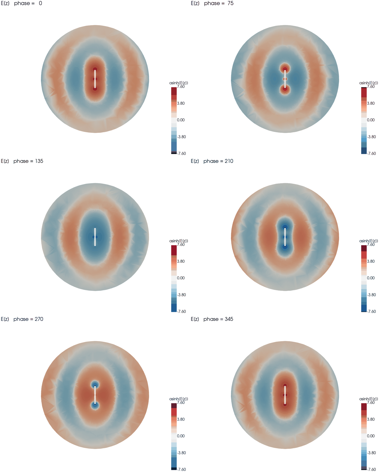
Electric Field Around the Dipole
The lumped port at the gap drives the two conductor arms. The electric field peaks near the feed and forms the familiar toroidal (doughnut-shaped) radiation pattern of a half-wave dipole, with the spherical absorbing boundary allowing energy to leave the domain as if into open space.
Simulation Configuration
Geometry & Mesh
Element Type:
Two cylindrical arms
Domain:
Spherical free space
Mesh Elements:
51,409
Element Order:
3rd (curved)
Degrees of Freedom:
332,066
Excitation & Frequency
Analysis Type:
Driven (freq. domain)
Frequency:
74.9 MHz
Wavelength:
≈ 4.0 m
Feed:
Lumped port
Reference Impedance:
50 Ω
Numerical Methods
Solver:
Palace (FEM)
Basis:
Nédélec (H-curl)
Preconditioner:
Geometric multigrid
Linear Iterations:
80
Precision:
Double
Boundary Conditions
Antenna Arms:
Perfect electric conductor (PEC)
Feed Gap:
Lumped port excitation
Outer Sphere:
Absorbing (far-field radiation)
Computational Performance
~39 s
Wall-Clock Time
A100
NVIDIA GPU
332K
Degrees of Freedom
3rd
Element Order
Simulation Results
−7.19 dB
Return Loss |S₁₁|
10.7 J
Stored Electric Energy
10.5 J
Stored Magnetic Energy
Interpreting the Numbers
Return loss of −7.19 dB means the antenna accepts the majority of the incident power at 74.9 MHz, with the remainder reflected back to the source — a realistic match for a simple thin-wire dipole against a 50 Ω feed.
Near-equal electric and magnetic energy (10.7 J vs 10.5 J) is the classic signature of operation close to resonance, where the dipole behaves as an efficient radiator rather than a reactive load.
The full complex port voltage and current are recovered, so the complete input impedance and phase response are available directly from the driven solve.
The Physics of a Half-Wave Dipole
Why Half a Wavelength?
A dipole radiates most efficiently when its total length is about half the operating wavelength. At λ/2 the current distribution forms a single half-sine along the conductor, the input reactance nearly cancels, and the antenna presents a mostly resistive impedance — making it easy to match and highly efficient. Here the ≈ 4 m wavelength (74.9 MHz) pairs with two quarter-wavelength arms to place the device right at this resonance.
Why a Full-Wave Field Solver?
Analytical formulas only capture idealized dipoles. Real designs have finite conductor thickness, feed structures, and nearby objects that shift resonance and reshape the radiation pattern. A full-wave finite-element solver like Palace resolves Maxwell's equations directly on the 3D geometry, so S-parameters, impedance, and near-fields reflect the actual hardware — not a textbook approximation.
Industrial Applications
Broadcast & Communications
Design and tune transmit/receive antennas for radio, TV, and telemetry links, predicting bandwidth and impedance match before building hardware.
Wireless & IoT Devices
Optimize compact antennas for phones, wearables, and IoT sensors where package constraints and detuning from nearby components are critical.
Aerospace & Radar
Characterize radiating elements and arrays for satellite links, avionics, and radar, including installed-performance effects on real platforms.
Quantum & RF Hardware
Extract resonances and coupling for RF control lines and readout structures in quantum devices, where precise electromagnetic modeling is essential.
Why NumericalAI for Electromagnetics
Powered by Palace — AWS's open-source, GPU-accelerated 3D finite-element solver for full-wave electromagnetics
Eigenmode, driven, and transient analysis — S-parameters, impedance, resonances, and near/far-field quantities in one workflow
High-order curved elements — accurate fields on curved conductors with fewer unknowns
Cloud GPUs on demand — full-wave solves in seconds to minutes, no local HPC cluster required
Business Value & ROI
NumericalAI brings production-grade electromagnetic simulation to an intuitive cloud interface — no solver installation, no cluster administration, no meshing expertise bottleneck.
Faster design cycles: sweep frequencies, tune geometry, and validate impedance match in minutes, so RF teams iterate on dozens of design variants before committing to a prototype build.
Ready to Simulate Your Antenna?
Run full-wave electromagnetic simulations with Palace on NumericalAI. Upload your Palace config.json and mesh, and get S-parameters and fields on cloud GPUs.
AI-Assisted GPU-Powered Simulations
© 2026 NumericalAI, all rights reserved. |Privacy Policy |Terms of Service |Executive brief |CEM vs HFSS |FAQ